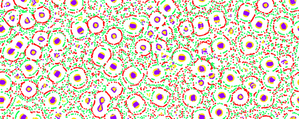
We're super excited to bring you Particle Life in Physion: a mesmerizing simulation where particles interact through simple attraction and repulsion forces, creating surprisingly organic patterns and behaviors. It's a beautiful demonstration of how complexity emerges from simplicity and it's really fun to play with.

What is Particle Life?​

Particle Life is a fascinating artificial life simulation that creates surprisingly organic behavior from simple rules. Different colored particles are scattered across space, each following attraction or repulsion rules toward other colors. Red particles might attract blues while repelling greens, creating an asymmetric web of interactions that leads to unexpected complexity.

Each particle has just three properties: a type (color), a position, and a velocity. From these simple ingredients and basic force rules, you get intricate, sometimes unexpected patterns that look almost alive. Particles cluster, spiral, orbit, and form dynamic structures. It's like watching microscopic organisms under a digital microscope!

The Magic of Emergence​

Particle Life belongs to a family of simulations that demonstrate emergent behavior where complexity arises from the interaction of individual agents following simple rules. This concept has inspired some of the most influential work in artificial life, including Craig Reynolds' Boids, which simulated flocking behavior, and Conway's Game of Life, which showed how four simple rules could create astonishing complexity.

The concept traces back to John Von Neumann's 1948 work on automata, where he explored whether we could build aggregates that could self-reproduce. Particle Life answers this question in its own way: while particles don't reproduce, they do organize, adapt, and create patterns that mirror phenomena we see in living systems.

What makes these simulations so compelling is their unpredictability. Through simple rules, researchers explore how emergent behavior creates systems that evolve and adapt over time. You might set up identical initial conditions except for one particle in a slightly different position, and watch entirely different patterns emerge—much like how tiny changes in nature can lead to vastly different outcomes.

Watch It in Action​

Check out our video tutorial showing Particle Life in action and learn how to create your own simulations in Physion:

How it works​

At its core, Particle Life is beautifully simple. Here's what makes it tick:

The Interaction Rules: Each color of particle has a relationship with every other color; it either attracts or repels them. These relationships are stored in a simple grid called an interaction matrix. For example, red might attract blue with a strength of +0.8, while blue repels red with -0.3. These asymmetric relationships create the magic: particles can chase each other in circles, form clusters, or flow like rivers.

The Force Calculation: Every frame, each particle looks at its neighbors and calculates forces based on their colors and distances. Particles that are too close always push apart, while particles at medium distances follow the attraction/repulsion rules. Particles far away ignore each other completely.

The Movement: Based on all these forces, each particle accelerates in a direction, moves to a new position, and gradually slows down due to friction. Without friction, they'd speed up forever; with too much, they'd stop moving entirely. The balance creates fluid, organic motion.

The Wrapping World: When a particle reaches the edge of the world, it wraps around to the opposite side—like the classic game Pac-Man. This creates an infinite, seamless space where patterns can flow continuously without hitting walls.

The Performance Trick: To simulate thousands of particles efficiently, the world is divided into a grid. Each particle only checks for neighbors in nearby grid cells rather than checking every single particle. This clever optimization makes real-time simulation possible without melting your computer.

Creating Your First Particle Life Simulation​

Ready to create your own artificial universe? Here's how to get started with Particle Life in Physion:

Step-by-Step Tutorial​

1. Open Physion and create a new scene
2. Change the background to black (optional, but provides better contrast for viewing the colorful particles)
3. Open the Tools menu and select Particle Life
4. A dialog box will appear—leave all default settings as they are for now, and click Execute
5. You'll see a new Particle Life Node added to your scene
6. Fit the node to your viewport so you can see everything clearly
7. Click the Start button to run the simulation

Watch as the particles begin to move and interact according to the default configuration.

Tweaking Parameters​

Now comes the fun part: experimentation! Select the Particle Life node and open the Property Editor. You'll find all the adjustable properties that control how particles behave. The simulation updates instantly as you make changes, allowing you to explore different patterns in real-time.

Here are the main settings you can adjust:

Tips for Discovering Interesting Patterns​

• Start simple: Try changing just colorCount first (3-10 colors work well). Then adjust forceStrength and beta—these have dramatic effects.
• The seed is your time machine: Found something amazing? Note the seed value and you can recreate it exactly. Want something new? Change the seed.
• Balance is key: Too much force strength or too little friction creates chaos. Too much friction or too little force creates boring, static patterns. The sweet spot is somewhere in between.
• Give it time: Some patterns take 30-60 seconds to fully develop. What looks random at first might evolve into beautiful structures.
• Try extremes: Set beta to 0.1 or 0.9. Set friction to 0.1 or 0.9. Extreme values often produce the most surprising results.

Common Pattern Types You Might Discover​

As you experiment, you'll encounter various emergent behaviors:

• Clustered blobs: Particles group into stable, slowly drifting clusters
• Orbital systems: Particles circle around each other like planets and moons
• Flowing rivers: Streams of particles flow in coherent patterns across the world
• Spiral galaxies: Rotating structures that maintain their shape while spinning
• Chaotic swarms: Constantly shifting, unpredictable particle clouds
• Stable lattices: Crystalline arrangements that barely move
• Chase patterns: One color perpetually chasing another in endless loops

Each pattern emerges from the same underlying rules—only the parameters and random seed differ. This is the beauty of emergent systems: infinite variety from finite rules.

Beyond Entertainment: Real Applications​

While Particle Life is incredibly fun to play with, these types of simulations have serious applications:

• Understanding biological systems: How cells organize, how proteins interact, how organisms coordinate
• Swarm robotics: Programming drones or robots to work together without central control
• Algorithm design: Creating optimization algorithms inspired by natural processes
• Art and visualization: Generating dynamic, organic visuals for games, films, and installations
• Education: Teaching complex systems, emergence, and computational thinking in an engaging, visual way

Final Thoughts​

Particle Life is all about play, exploration, and seeing what emerges. You don't need to understand advanced mathematics or computer science—just try things, see what happens, and enjoy the visuals. It's fast, accessible, and filled with surprises.

The remarkable thing about Particle Life—and emergent systems in general—is that no one programmed the spirals, clusters, or orbits you'll see. These patterns emerge naturally from the interaction of simple rules. In a way, you're not just running a simulation; you're creating conditions for artificial life to evolve and organize itself.

So fire up Physion, add a Particle Life node, and start experimenting. Who knows what patterns you'll discover? The only limit is your curiosity.

Have fun messing around, and let us know if you discover something wild, beautiful, or totally unexpected!

Physion is now equipped with audio support, thanks to the integration of the Tone.js library. In this blog post, we'll briefly explain what Tone.js is and how you can use it to enhance your Physion projects with audio.

While most of Physion's features are easily accessible through a user-friendly graphical interface, audio support, at least for now, is accessible exclusively through scripting. This means that you won't find a convenient UI tool for adding an "audio component" to your scenes. Instead, you'll need to import the audio library into your scripts and use it to create various sounds and audio effects. Let's dive into the process.

Tone.js​

Before we explore how to use Tone.js in your scripts, let's briefly introduce the library.

Tone.js is a JavaScript library designed for audio and music creation on the web. It offers a framework for synthesizing and processing sound, making it easier for developers to build interactive music and audio applications directly in the browser.

Basic usage​

Let's consider a very basic example of how you can utilize Tone.js in your scripts.

In the following very basic example, we'll create a NodeScript responsible for playing a sound whenever another object collides with it.

class BlipPlayer {

    constructor(node) {
        this.node = node;
        this.initialized = false;
    }

    async initialize() {
        const Tone = await physion.utils.importTone();
        this.synth = new Tone.PolySynth(Tone.Synth).toDestination();
    }

    update(delta) {
        if (!this.initialized) {
            this.initialize();
            this.initialized = true;
        }
    }

    onBeginContact(bodyNode, contact) {
        if (this.synth && contact.IsTouching()) {
            this.synth.triggerAttackRelease("C4", "32n");
        }
    }
}

Let's break down what this NodeScript does:

As with all NodeScripts, the constructor is called with one argument: the Node that the script is going to be attached to. It's the responsibility of the script to store a reference to this Node so that a later time it can reference it. Also, in the constructor we're initializing a data member named initialized to false to denote that the script hasn't yet initialized.

As the name suggests, the initialize method is responsible for initializing the NodeScript. In this particular case, we need to import the Tone.js library and when this is done then create our synth object. Later on we'll use the synth object to play our sounds.

In the update method, we simply check if we have already initialized and if not then we call our initialize method.

Finally, in the onBeginContact method we check if the contact is touching and if we have already created our synth and if both of these conditions are true then we go ahead and play a note via our synth object. In this example we're playing the C4 note but any other note could be used instead.

The above example serves as a foundation for understanding how Tone.js can be integrated into your projects, allowing you to create diverse audio experiences within your scenes. As you explore audio support in Physion further, you'll discover many more possibilities for enhancing your creations with audio.

In Tone.js page you can find many more examples on how this library can be used in order to produce various sound effects.

Stay tuned for more in-depth tutorials and creative use cases for audio support in Physion with Tone.js!

A feature that up until now was missing from Physion was the ability to create graphs. With graphs we can easily interpret data and better understand how properties of objects participating in our simulation change over time.

Graph Tool​

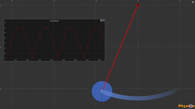
You can create graphs using the graph tool. Once the tool is selected, you can click on any body in your scene to create a graph for. After you select a body using the graph tool, a new panel will appear in your Scene:

The header of this panel contains the title of the graph (e.g. "Linear Velocity") and two buttons on its right side. This panel will contain the graph of the selected body. By defult the Linear Velocity vs Time will be plotted.

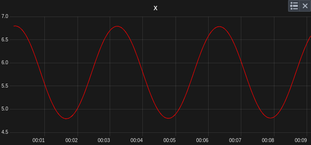
At the top right of the graph panel you can find two buttons; the select button will select the graph and make it available for changes in the property editor and the close button will remove the graph from the Scene.

GraphNode​

The underlying node for graphs is the GraphNode. As with all other types of nodes, you can edit its properties via the Property Editor. These properties are the following:

Up until now, the physics engine used by Physion was Box2D. Box2D is an open source 2D physics engine written in C++ and it is used in many games and apps.

Although Box2D is a mature physics engine with many features, it doesn't "natively" support fluid simulation. After some research on the web, I came across LiquidFun. As mentioned in LiquidFun's website:

LiquidFun is an extension of Box2D. It adds a particle based fluid and soft body simulation to the rigid body functionality of Box2D.

As it turns out, transitioning from Box2D to LiquidFun is quite easy. All the features supported in Box2D are also supported in LiquidFun so there's no need for any major code changes when switching to LiquidFun.

Although LiquidFun supports a rich set of features, we will start simple; the transition to LiquidFun will have one simple goal: Allow the user to convert a rigid body into a liquid or an elastic (soft) body.

When a rigid body is "liquified" or "elastified" it will be removed from the Scene and in its place a new node will be added. This new node will contain all the particles representing the liquified or elastified body.

Liquify / Elastify Tools​

The first change that was implemented was to add two new tools in the toolbars.

These two new tools are:

• Liquify Tool
• Elastify Tool

The user can select any of these tools and then click on a rigid body in the Scene in order to liquify or elastify it.

Some notes:

• The visual feedback of these new tools is minimal (just a single sprite)
• These tools will only allow liquifying/elastifying a single body at a time (i.e. single click selection)

Liquify / Elastify Commands​

Both of these new commands will work in a very similar manner:

• They will create a new LiquidNode or ElasticNode using the selected body's: transformed shape, linear velocity and fill color.
• They will remove the selected body (and its dependencies) from the Scene.
• They will insert the new LiquidNode or ElasticNode in the Scene.

Note that in contrast with most commands that append new nodes in the Scene, these commands will insert the new Node instead. The reason this is done is to have all liquids and soft bodies stacked behind rigid bodies (which looks more realistic).

Scene Updates​

The main change in the Scene node is the addition of a particle system. This means that when a new Scene is constructed a new particle system will be constructed with it. All liquids and elastic bodies that will be created by the user will belong to this particle system. A particle system has many options that can be defined but for the time being these options will not be exposed to the user nor they will be saved in the Scene (this might be done in the future).

Also, a new property was added in the Scene. Its name is particleIterations and its default value is 3. The higher this value is the better (more accurate) the particle simulation will be.

ParticleGroupNode​

The ParticleGroupNode serves as the base class for both LiquidNode and ElasticNode.

As the name suggests, this node represents a group of particles.

Each particle is round, has a fixed rotation and has the following properties:

• Position
• Velocity
• Color

Because both of the liquify and elastify commands produce lots of particles (typically in the range of thousands) we need to better handle how the ParticleGroupNode is saved. In order to solve this it was decided to use (lz) compression when packing the Scene.

Some general key points for the ParticleGroupNode are:

• Its x, y and angle properties are always zero and cannot be changed.
• Its bounding rectangle is defined by the positions of the particles it contains.

Selection​

As mentioned above, the ParticleGroupNode is a group of particles. For the time being, the user can only select the group as a whole and individual particles within the group cannot be selected.

Rendering​

Ideally, for rendering the particles we would use shaders but since shaders are not yet supported in Physion we will use a simpler approach. To render each particle a single sprite will be used.

The texture for this sprite looks like:

Limitations​

• A ParticleGroupNode cannot be moved or mirrored.

Future Work​

• Use shaders to better visualize liquid and elastic bodies.
• Expose more LiquidFun properties (Particle System/Group) in the UI.

A new (BodyNode) property was recently added in Physion.

Its name: Gravity Scale (gravityScale).

As the name suggests, the gravityScale property of a body can be used to "scale" the gravitational attraction applied to it. In other words, the gravityScale allows you to specify a different gravity for each body.

By default, the value of this new property is 1.0 meaning that the Scene's gravity will be applied to the body. If you change this value to say 0.5 then only half of the Scene's gravitational force will be applied to the body. If you want to make a body float (i.e ignore gravity) you can set a gravity scale of 0. To make a balloon-like body you can set its gravityScale to a negative number.

In the video below you can see the gravity scale in action:

Note that the minimum value of this property is -1 and its maximum value is +1.

Using this new property and some minimal scripting, the user can easily create gravity pads which are very useful in marble races and other similar simulations.

Recently, a feature request was made in Physion's Discord Server: "Add the ability to visualize the trajectory of an object". This functionality was already implemented in the old version of Physion as you can see in the video below:

Unfortunately (and for the time being) the web version of Physion doesn't natively support tracers. The goods news is that we can implement the tracer functionality using scripting.

The Tracer Script​

We're going to create a NodeScript (i.e. a script that gets attached to a Node) to implement the tracer functionality.

Let's start with the constructor:

 class Tracer {

    constructor(node) {
        this.node = node;
        this.initialized = false;

        this.trajectory = [];
        this.maxTrajectorySize = 100;

        if (typeof physion !== "undefined") {
            this.graphics = physion.utils.createGraphics();
            this.lineStyle = physion.utils.createLineStyle(0);
            this.fillStyle = physion.utils.createFillStyle(0xff0000);
        }

        this.tracerRadius = 0.1;
    }

  // ..

}

In the constructor we initialize the data members of the class that we're going to use:

The update() method of the script is shown below:

update(delta) {
    if (!this.initialized) {
        this.initialized = true;
        const scene = this.node.findSceneNode();
        if (scene) {
            scene.layers.foreground.addChild(this.graphics);
        }
    }

    this.updateTrajectory();
    this.drawTracer();
}

First, we use our initialized data member to perform a 'one-off' initialization task: Add our graphics to the foreground layer of the scene (that our node belongs to). In order to retrieve the scene that our node belongs to, we use the findscenenode method.

After initialization is performed, the script keeps repeating the following:

• Updates the trajectory array
• Draws the tracer

The updateTrajectory() method is responsible to update our trajectory array in each update. It does that by pushing the latest position of our node to the array. It also makes sure that this array doesn't grow infinetely: If the size of the trajectory array gets bigger than maxTrajectorySize then old positions will get removed.

updateTrajectory() {
    this.trajectory.push(this.node.getPosition());
    while (this.trajectory.length > this.maxTrajectorySize) {
        this.trajectory.shift();
    }
}

Finally we call the drawTrajectory helper which will use the trajectory array to draw a series of circles thus visualizing the trajectory of our node:

drawTracer() {
    if (this.graphics && this.fillStyle) {
        this.graphics.clear();
        this.trajectory.forEach((point, i) => {
            this.fillStyle.alpha = (i + 1) / this.trajectory.length;
            physion.utils.drawStyledCircle(this.graphics, point.x, point.y, this.tracerRadius, this.lineStyle, this.fillStyle);
        });
    }
}

Using the Tracer Script​

The Tracer script is available in the Assets Browser. To use it simply drag and drop the script onto the node to create the tracer for.

You can also see the tracer script in action in this sample scene.

Future Work​

• Add the ability to trace any point on an object (and not just its center as presented in this solution).
• Add a TracerNode (and the corresponding UI) to allow creating tracers natively (i.e. without a custom script)
• More customization (e.g. gradient color)